Moderation
Abstract
When moderation is present, the strength or even the direction of a relationship between two constructs depends on a third variable. In other words, the nature of the relationship differs depending on the values of the third variable. As an example, the relationship between two constructs is not the same for all customers, but differs depending on their income. As such, moderation can (and should) be seen as a means to account for heterogeneity in the data.
Brief Description
Moderation describes a situation in which the relationship between two constructs is not constant but depends on the values of a third variable, referred to as a moderator variable. The moderator variable (or construct) changes the strength or even the direction of a relationship between two constructs in the model. For example, prior research has shown that the relationship between likeability of a corporation and customer loyalty differs as a function of the customers’ switching costs. More precisely, switching costs have a pronounced negative effect on the likeability-loyalty relationship: the higher the switching costs, the weaker the relationship between likeability and loyalty. In other words, switching costs serve as a moderator variable that accounts for heterogeneity in the likeability-loyalty link. Thus, this relationship is not the same for all customers, but instead differs depending on their switching costs. As such, moderation can (and should) be seen as a means to account for heterogeneity in the data.
Moderating relationships are usually hypothesized a priori by the researcher and are specifically tested. The testing of the moderating relationship is done by assessing the effect of the interaction term (i.e., the product of the moderator and predictor variable), which indicates whether changes in the moderator increase or decrease the strength of the focal relationship. A simple slope plot (see below) further helps to assess the moderation effect.
Hair et al. (2022) describe PLS-SEM moderator analysis in more detail. Moderation can also be combined with mediation in PLS-SEM in order to carry out a moderated mediation or conditional process analysis (Cheah et al., 2021; Hair et al. 2022; Sarstedt et al. 2020).
Moderation in SmartPLS
Moderation model generation (two-way interaction) and results computation
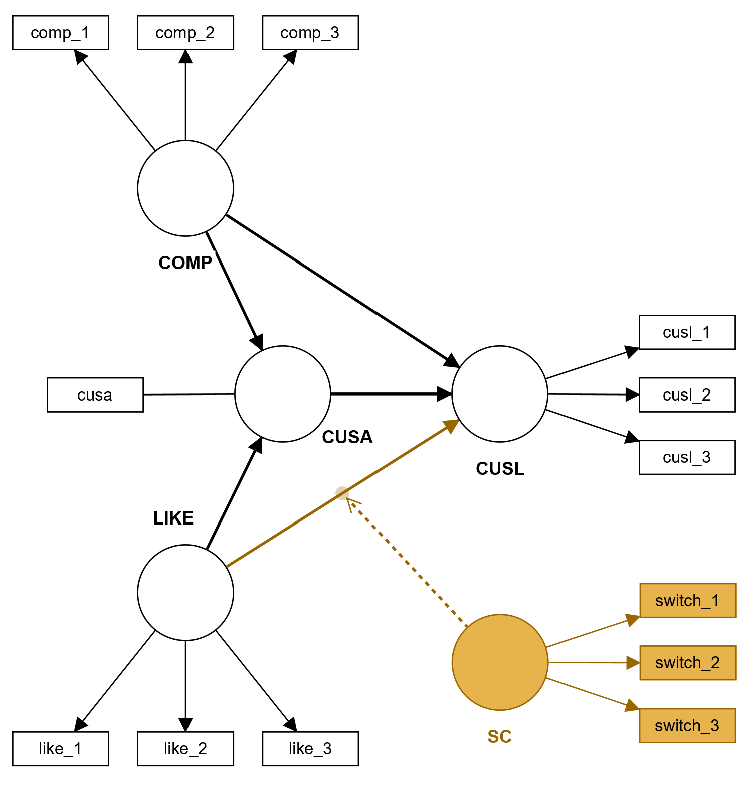
Include the moderator construct in the PLS path model (e.g., by including a single-item or a multiple item construct). Next, add a relationship from the moderator to the path relationship between two constructs you want to moderate. The following figure shows how the switching costs construct moderates the relationship from likeability to loyalty in this two-way interaction example for the corporate reputation model (see also Hair et al., 2022).

When calculating the results, SmartPLS 4 automatically adds a relationship from the moderator to the dependent variable of the moderated relationship - regardless of whether the relationship was extra included in the model or not (as in the figure above). This is a statistical requirement to get correct results for the moderation.
To compute the moderation results, SmartPLS performs the two-stage approach (see also Becker et al., 2018), which uses the latent variable scores of the latent predictor and latent moderator variable from the main effects model (without the interaction term). These latent variable scores are saved and used to calculate the product indicator for the second stage analysis that involves the interaction term in addition to the predictor and moderator variable.
Two important notes:
- If standardized, unstandardized, or mean centered is selected in the options when starting the PLS-SEM algorithm, then the correspondingly generated latent variable scores of the constructs are used to calculate the interaction term in the second stage.
- The interaction term (latent variable) is left as it is when entering the final regression of the moderator model (i.e., independent and moderator variables as well as interaction term on the selected dependent variable). Hence, it is not standardized which would bias the results.
Furthermore, the use of binary moderators requires special care and additional considerations. For moderation analysis, it is important that the binary variable be dummy-coded as 0/1 and not, for example, as 1/2, because the reference point for result interpretation is always zero. When researchers and practitioners use such a binary moderator variable representing two different categories in a path model, the routine standardization of all input variables in PLS-SEM makes it difficult to interpret a standardized binary variable because the reference point (i.e., mean value) lies somewhere between the two categories and does not represent a meaningful value (i.e., no category). Although this reference point is not interpretable, the model is still estimated correctly, and manual calculations can be used to identify correctly interpretable effects. Becker et al. (2022) explain how results can be manually corrected for interpretation when a binary moderator is used.
Three-way and more way interaction
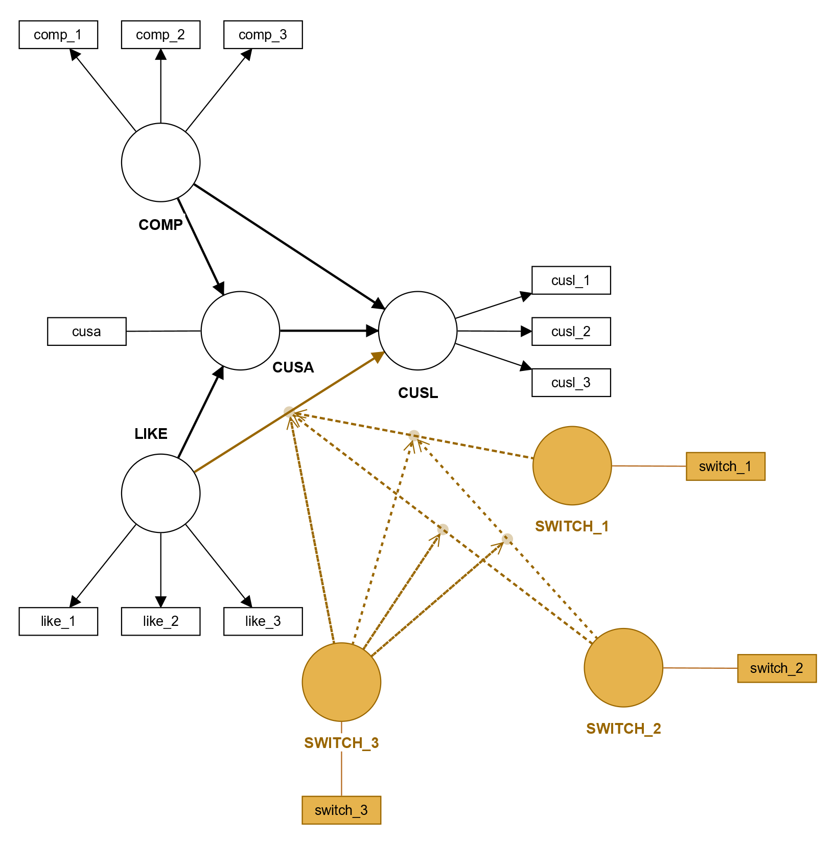
SmartPLS 4 enables the calculation multi-way interactions such as the three-way interaction (and higher). One only has to draw a path from the additional moderator on the interaction offset already present in the model. Thus, the moderation of a moderation is mapped. Any additional relationships required (for example, from the additional moderator to the dependent variable of the moderated relationship) are again automatically added by SmartPLS. The calculations are analogous to the description of the two-way interaction. Becker et al. (2022) provide further explanations on how to conduct a multi-way interaction analyses in PLS-SEM. The following figure shows a three-way interaction using the example of the coporate reputaton model.

Simple slope plot
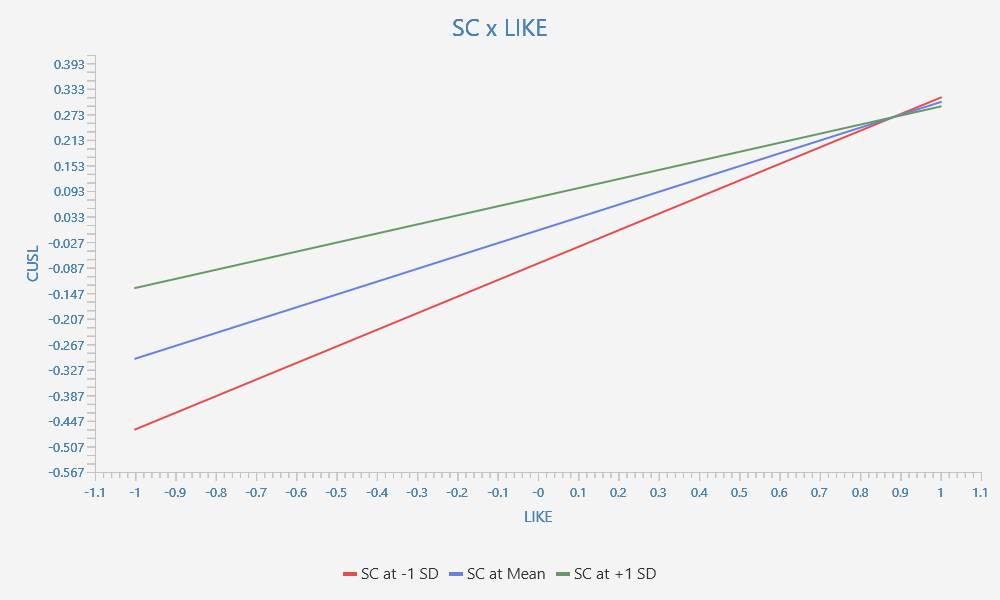
A typical moderator analysis results representation uses simple slope plots. SmartPLS provides simple slope plots in the results report. The following figure shows a simple slope plot for the relationship from likeability to loyalty, which is moderated by switching costs in the corporate reputation model example (see also Hair et al., 2022).

It shows that for high switching costs (i.e., +1 standard deviation above the mean; green line) we have a weaker relationship (i.e., flatter line) between CUSA and CUSL than when we have low switching costs (i.e., -1 standard deviation below the mean; red line), which slope is steeper. It illustrates that reductions in likeability translate stronger into reductions in loyalty for customers perceiving lower switching costs than for those perceiving high switching costs.
References
- Becker, J.-M., Cheah, J. H., Gholamzade, R., Ringle, C. M., and Sarstedt, M. (2023): PLS-SEM’s Most Wanted Guidance, International Journal of Contemporary Hospitality Management, 35(1), pp. 321-346.
- Becker, J.-M., Ringle, C. M., and Sarstedt, M. (2018). Estimating Moderating Effects in PLS-SEM and PLSc-SEM: Interaction Term Generation x Data Treatment Journal of Applied Structural Equation Modeling, 2(2), pp. 1-21.
- Cheah, J. H., Nitzl, C., Roldán, J. L., Cepeda Carrión, G., and Gudergan, S. P. (2021). A Primer on the Conditional Mediation Analysis in PLS-SEM. ACM SIGMIS Database: the DATABASE for Advances in Information Systems, 52, 43-100.
- Hair, J. F., Hult, G. T. M., Ringle, C. M., and Sarstedt, M. (2022). A Primer on Partial Least Squares Structural Equation Modeling (PLS-SEM), 3rd Ed., Sage: Thousand Oaks.
- Sarstedt, M., Hair, J. F., Nitzl, C., Ringle, C. M., and Howard, M. C. (2020). Beyond a Tandem Analysis of SEM and PROCESS: Use of PLS-SEM for Mediation Analyses!. International Journal of Market Research, 62(3), 288-299.
- More literature ...
Cite correctly
Please always cite the use of SmartPLS!
Ringle, Christian M., Wende, Sven, & Becker, Jan-Michael. (2024). SmartPLS 4. Bönningstedt: SmartPLS. Retrieved from https://www.smartpls.com

