
Understanding 'n/a' Results in SmartPLS: Causes and Solutions
SmartPLS shows n/a for a parameter (e.g., path coefficients, loadings, weights) when there is no possible solution for it. This is expected behavior, not a bug.
It usually happens during bootstrapping: one or more bootstrap samples lead to an invalid solution, meaning no solution could be calculated for the model or some of its parts. The result table then shows n/a for the problematic parameter. If an n/a occurs across all bootstrap samples, the mean and standard deviation of the bootstrap distribution cannot be calculated, so these outcomes show n/a as well.
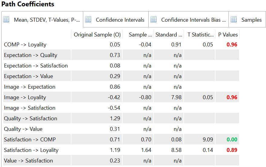
To reproduce the screenshot: run SmartPLS, open the ECSI model, select the data set with 98 observations and start consistent bootstrapping with the default settings.
SmartPLS does not filter out invalid bootstrap solutions, because that would bias your results (see the next section). What typically causes them depends on the algorithm you use.
Why invalid bootstrap solutions are not filtered out
Inadmissible solutions always indicate a problem with the data or the model. The missing results make you aware of the problem, so you can address it and arrive at an adequate solution.
Filtering out inadmissible solutions would also distort the sample distribution that bootstrapping generates. The result would only consider the "good" bootstrap solutions, so the bootstrapping routine may underestimate the actual variability of the parameter estimate (e.g., its standard error). This can lead to incorrect inferences from the model and the data (e.g., errors in the significance assessment).
Common causes by algorithm
When you use consistent PLS-SEM (PLSc-SEM) bootstrapping
Why it happens. The consistent PLS-SEM (PLSc-SEM) algorithm corrects the correlations of reflective constructs to make the results consistent with a factor model (Dijkstra and Henseler, 2015; Dijkstra and Schermelleh-Engel, 2014). For this, it uses rho_A, a reliability measure specific to the PLS-SEM context (Dijkstra and Henseler, 2015). This reliability statistic is known to be consistent in PLS-SEM: it approaches the true reliability under common regularity conditions of a common factor model and as sample sizes increase to infinity.
However, rho_A may produce inadmissible solutions in smaller samples and when common factor assumptions do not hold (e.g., when the construct follows a composite model; e.g., Rigdon 2016; Rigdon, Sarstedt, and Ringle, 2017; Sarstedt et al. 2016). The reliability estimate can then fall outside the permissible range of 0 to 1 (Takane and Hwang, 2018):
- If it is negative, the correction does not work at all, because it requires the square root of rho_A, which is not defined for negative values.
- Extreme positive values can also cause estimation problems when the corrected correlations fall outside the interval −1 to 1.
The problem has been compared to Heywood cases in CB-SEM, where the method estimates negative variances (which are impossible).
What to do. PLSc is very strict about the common factor model assumptions; deviations from them likely lead to estimation problems and thus inadmissible solutions.
- Revisit the common factor model assumption of your reflective constructs. If appropriate, treat and estimate the constructs as composites.
- If you assume common factor models, use a larger sample size. This is a simple way to avoid these problems.
When you use standard PLS-SEM bootstrapping
Inadmissible solutions occur much less often with standard PLS-SEM algorithms than with PLSc-SEM. They are almost always associated with either:
- (a) almost perfect collinearity in the model, or
- (b) a variable with zero variance.
Why it happens. Both problems may not appear in the original data but can manifest during bootstrapping. Bootstrapping is a random process that draws observations from the original sample with replacement to create a bootstrap subsample. The results for a parameter estimate across all subsamples represent the sample distribution. Because the process is random, some subsamples may show extreme characteristics.
Collinearity. Strong multicollinearity in the overall sample may become perfect collinearity if only those observations are drawn that are perfectly collinear. Cure the collinearity problem or try to increase the sample size.
Variance close to zero. Inadmissible solutions may occur if the model contains variables with a variance close to zero (i.e., the same value for almost every respondent). If a variable contains very similar responses, a subsample may contain only observations with the same value, so the variable has zero variance in that subsample. Standardization in PLS-SEM divides the values by the variance of the variables, and a division by zero leads to an inadmissible solution. This is likely to occur:
- in a very homogeneous group in which some variables have little variance,
- if you include the grouping variable as an indicator in the model and run a multigroup analysis (after grouping, this variable has only one value and therefore no variance),
- with dummy variables (i.e., zero-one variables) for which one category is very rare.
The problem is inflated in small samples, where drawing such a subsample is more likely than in large samples.
What to do. Check your model for variables with low variance and, if possible, exclude them or increase the sample size.
When you use PLS-SEM (or PLSc-SEM) fit indices
Some PLS-SEM fit indices are of limited general applicability for model evaluation. For example, they are not defined for models with repeated indicators (e.g., when estimating higher-order models in PLS-SEM). Such models include perfect correlations of 1 in the indicator correlation matrix, because the same indicator is used twice and correlates perfectly with itself. In this case, some fit indices cannot be calculated.
When you use CB-SEM bootstrapping
Why it happens. CB-SEM may not generate all requested bootstrap samples, so fewer samples are used for the calculations than you specified. CB-SEM relies on convergence, where the model reaches a stable solution. Some bootstrap samples may not converge, especially with problematic data patterns or model misspecification. In these cases, the algorithm terminates early for that sample and excludes it from the bootstrap results, which reduces the number of bootstrap samples.
What to do. Fewer bootstrap samples than requested do not necessarily invalidate the results. Thoroughly assess the available samples and carefully consider the reasons for the reduced count to ensure the validity and reliability of your findings.
References
- Dijkstra, T. K., & Henseler, J. (2015). Consistent partial least squares path modeling. MIS Quarterly, 39(2), 297–316.
- Dijkstra, T. K., & Schermelleh-Engel, K. (2014). Consistent partial least squares for nonlinear structural equation models. Psychometrika, 79(4), 585–604.
- Takane, Y., & Hwang, H. (2018). Comparisons among several consistent estimators of structural equation models. Behaviormetrika, 45(1), 157–188.
- Sarstedt, M., Hair, J. F., Ringle, C. M., Thiele, K. O., & Gudergan, S. P. (2016). Estimation issues with PLS and CBSEM: Where the bias lies! Journal of Business Research, 69(10), 3998–4010.
- Rigdon, E. E., Sarstedt, M., & Ringle, C. M. (2017). On comparing results from CB-SEM and PLS-SEM. Five perspectives and five recommendations. Marketing ZFP, 39(3), 4–16.
- Rigdon, E. E. (2016). Choosing PLS path modeling as analytical method in European management research: A realist perspective. European Management Journal, 34(6), 598–605.
- More literature ...